test-3-maple.mw

Introduction 

This web page is a transcript of an active Maple Worksheet, which you may download and execute from the classroom computer, any time the room is free.  Download the .mw file test-3-maple.mw, by right-clicking and choosing "Save..." from the pop-up menu.  Save it on the Desktop or anywhere convenient.  Then open it up for a live session. 

Load the Needed Packages 

with(plots); -1 

#s 1 and 2 

int(int(8*x*y, y = sqrt(3)*x .. exp(x^2)), x = 0 .. 1) 

-4+exp(2) 

`+`(int(int(8*x*y, x = 0 .. y/sqrt(3)), y = 0 .. 1), int(int(8*x*y, x = sqrt(ln(y)) .. y/sqrt(3)), y = 1 .. sqrt(3))+int(int(8*x*y, x = sqrt(ln(y)) .. 1), y = sqrt(3) .. exp(1)))
 

-4+exp(2) 

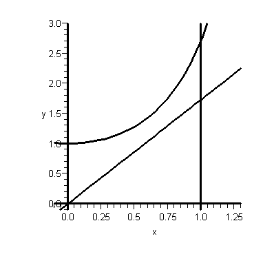
eplot := plot(exp(x^2), x = -.1 .. 1.3, y = -.1 .. 3, color = black, thickness = 2); -1; %; -1 

lineplot := plot(sqrt(3)*x, x = -.1 .. 1.3, y = -.1 .. 3, color = black, thickness = 2); -1; %; -1
 

xis1plot := implicitplot(x = 1, x = -.1 .. 1.3, y = -1 .. 3, color = black, thickness = 2); -1; %; -1
 

xis0plot := implicitplot(x = 0, x = -.1 .. 1.3, y = -1 .. 3, color = black, thickness = 2); -1; %; -1
 

yis0plot := implicitplot(y = 0, x = -.1 .. 1.3, y = -1 .. 3, color = black, thickness = 2); -1; %; -1
 

display([eplot, lineplot, xis1plot, xis0plot, yis0plot]) 


Plot 


Matthew Remembered this Was a Homework Exercise. 

int(int(x/(x^2+y^2), x = 1 .. 2), y = 0 .. 1) 

-1/2*ln(2)-1/4*Pi+1/2*ln(5)+2*arctan(1/2) 

evalf(%) 

.6000424200 

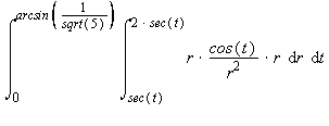
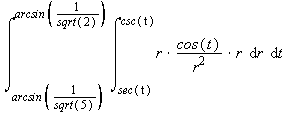
Getting this problem to work with polar coordinates was difficult, because the region didn't lend itself to easy description in polar coordinates.  But once you get the knack for describing horizontal and vertical lines in polar coordinates, with inverse trig functions, the range of values for r  isn't that difficult.  We're just not used to thinking this way, in polar coordinates. 


int(int(cos(t), r = sec(t) .. 2*sec(t)), t = 0 .. arcsin(1/sqrt(5)))+int(int(cos(t), r = sec(t) .. csc(t)), t = arcsin(1/sqrt(5)) .. arcsin(1/sqrt(2)))
 

2*arcsin(1/5*5^(1/2))+1/2*ln(5)-1/2*ln(2)-1/4*Pi 

evalf(%) 

.6000424205 

int(int(cos(t), r = sec(t) .. 2*sec(t)), t = 0 .. arcsin(1/sqrt(5))) 

arcsin(1/5*5^(1/2)) 

int(int(cos(t), r = sec(t) .. csc(t)), t = arcsin(1/sqrt(5)) .. arcsin(1/sqrt(2))) 

1/2*ln(5)+arcsin(1/5*5^(1/2))-1/2*ln(2)-1/4*Pi 

arcsin(1/sqrt(5)) 

arcsin(1/5*5^(1/2)) 


Number 5 

int(int(int(x^3+x*y^2, z = 0 .. 1-x^2-y^2), y = 0 .. sqrt(1-x^2)), x = 0 .. 1) 

2/35 


>